From docs/usage.md
How to use it
Everything you need to run the project: on your Mac (the web app or the command line), or on a cloud GPU with the notebooks. For what each part does inside, see Understanding the components; for what was measured, see Analysis.
Three ways to use it
| What it is | Best for | |
|---|---|---|
Web app · python3 app/server.py |
A local, step-by-step studio in your browser with explanations and live charts | Learning how it works, experimenting |
Command line · python3 full-model.py |
Runs the whole pipeline in one go | Long training runs |
| Notebook on Colab or Kaggle · Open in Colab | The same steps on a free cloud GPU; brings the model home as a zip | Bigger or longer training runs, or no Mac |
Made for Apple Silicon
- Trains on the Mac GPU. The device is picked automatically, and on M-series Macs that's the GPU through
PyTorch's Metal backend (MPS). The app and the script both show it at startup:
Training on device: mps (float32). - No extra setup. The standard
pip install torchalready includes Metal support on macOS. - Full precision on MPS. Training uses float32 on the Mac. Mixed precision is only switched on for CUDA, where it's well supported.
- Unified memory. Even the Large preset (124M parameters, about 2 GB to train) fits comfortably on a 16 GB Mac. The app checks the memory before building a model that wouldn't fit.
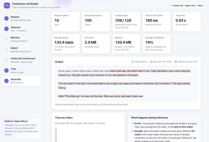
- Measured speed. On an M5 with 16 GB, the default model trains at about 2 steps per second (32 × 128 tokens per step, measured with the original 128-token window). The Quick preset (2,000 steps) takes roughly 20 minutes and brings the validation loss from 10.8 down to about 4.6. The full run (20,000 steps) takes several hours. Generation with the KV cache runs at about 130–150 tokens per second for the default model.
It also runs on an Nvidia GPU (CUDA, with mixed precision) or the CPU, but the Mac is what it's built and tested on.
Check that PyTorch can see your Mac's GPU:
python3 -c "import torch; print('MPS available:', torch.backends.mps.is_available())"
Quick start (Mac)
Requires an Apple Silicon Mac (M1 or later) and Python 3.9+.
git clone https://github.com/a-ramakrishnan/tinystories-ARM-model.git
cd tinystories-ARM-model
pip install -r requirements.txt
Web app (recommended)
python3 app/server.py
It opens http://127.0.0.1:8000 in your browser. The sidebar walks through seven steps:
- Dataset: add one or more datasets by name or link, or from the gallery of public datasets. Check validates a dataset before anything is downloaded. With several, choose whether batches mix them by size or equally.
- Tokenize: see how BPE works through examples (common words, rare words, numbers, capitals, emoji), try your own text, then tokenize your training data.
- Batches: a worked example shows how one window becomes many next-token exercises; then sample a real batch (and see which datasets it came from).
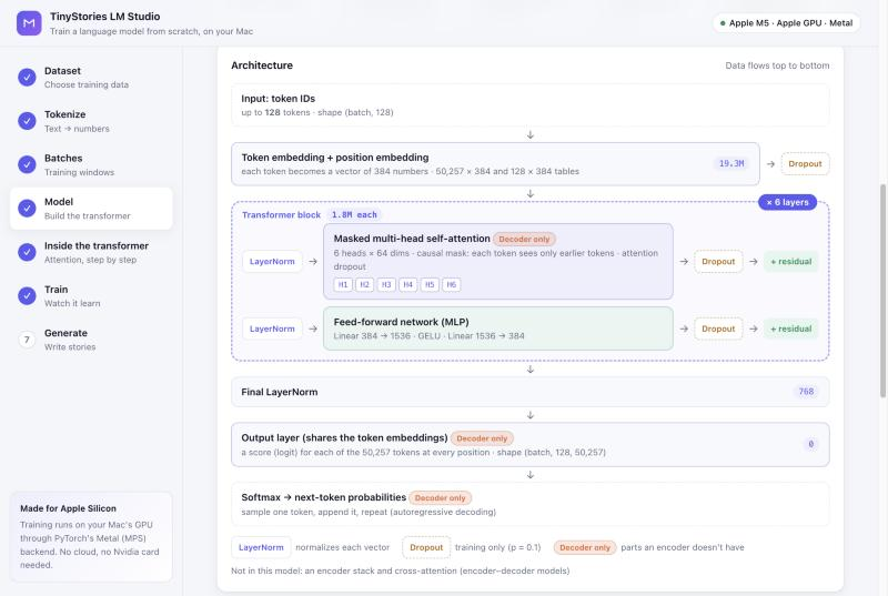
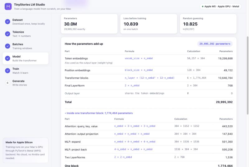
- Model: pick a size preset (Tiny 16M, Small 30M, Medium 51M, Large 124M) or set layers, heads and embedding size yourself, with a live parameter estimate. Building shows the architecture diagram, the input and output token counts, and how every parameter adds up.
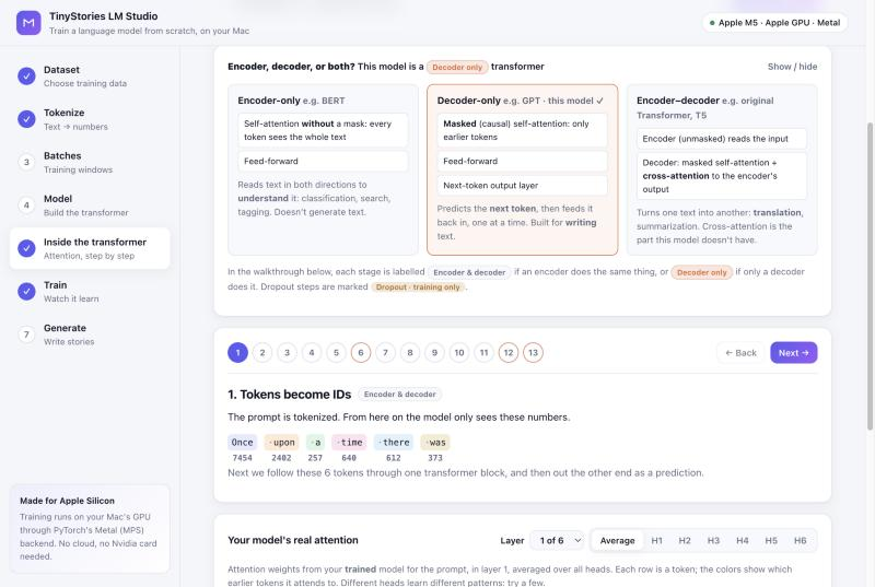
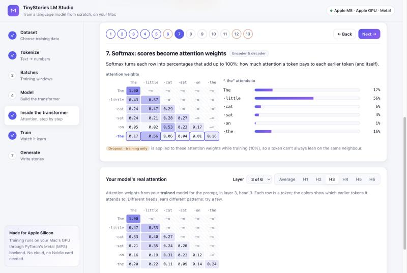
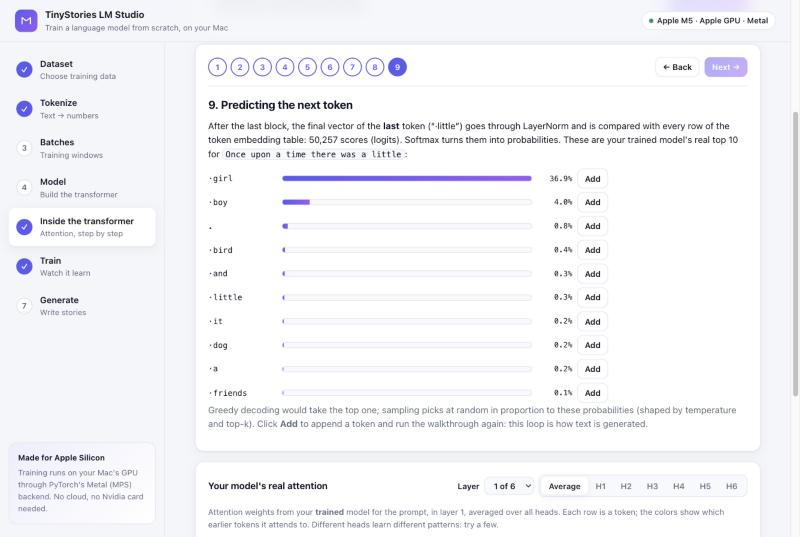
- Inside the transformer: compare encoder-only, decoder-only and encoder–decoder models, then walk a prompt through a whole transformer block and out to the next token in 13 stages, and explore your model's real attention heatmaps by layer and head. The Explorer (switch at the top of the step) draws your model's real numbers for the whole model at once, in two looks: - Flow (the default): ribbons carry every token from the embedding into each head's Q, K and V, through the chosen head's attention, down into the feed-forward layer and back, past the other blocks, and out to the next-token probabilities. ▶ Play the data flow follows one token through the whole model: block 1 step by step, then each later block's attention and feed-forward, with the diagram moving to each block as the token reaches it, and finally the prediction. It lights only the parts that act on the token, moves particles along its ribbons and explains each step with the real numbers; pause with space, step with ← →, jump to a block with the block arrows, or pick the token to follow. - Diagram: the numbers themselves, in two bands (attention, then feed-forward): embedding, query, key and value strips, the attention matrix as scores, mask or softmax (click a cell for its calculation), the feed-forward activations or the experts' router.
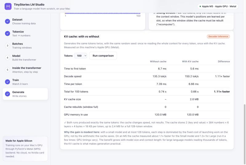
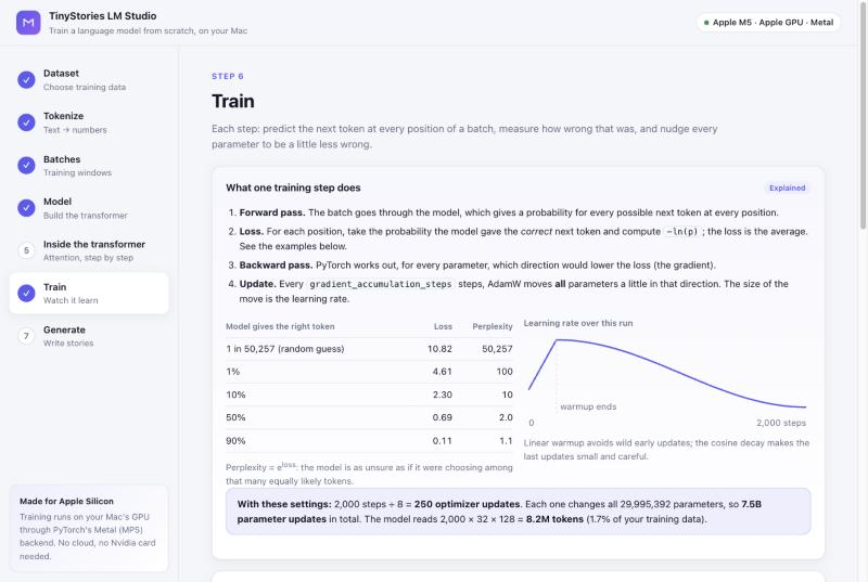
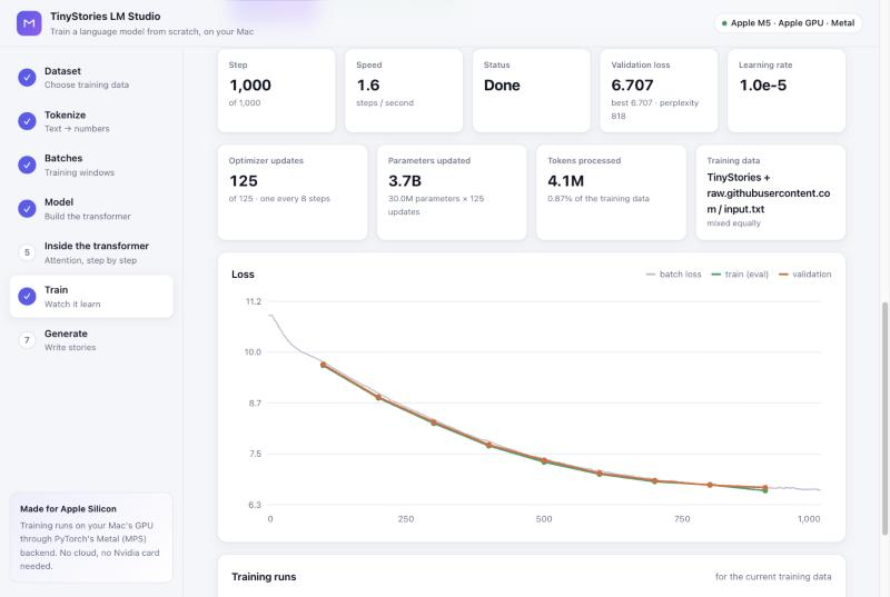
The next-token probabilities are for the token you follow or click (the last one otherwise); for an earlier token, the real next token is marked ✓ with the probability and rank the model gave it. Both views have head and block controls, sampling sliders for those probabilities, an explanation for every part, Full screen (Esc to leave), a logit lens table (what the model would predict after each block), and, when you click a token's name, a table that follows it through every block. 6. Train: see what one training step does, how loss relates to probability, and the learning-rate schedule; then train and watch loss, speed, optimizer updates, parameters updated and tokens processed. Every run is kept in a history table. 7. Generate: text streams in token by token, colored by the model's confidence, with tokens used, time to first token, decode speed, KV cache size, GPU memory and a per-token timing chart. Switch the KV cache on or off, or run a side-by-side comparison.
Options: --port 8080 to use another port, --no-browser to skip opening a browser tab. A step can be
opened directly with a link such as http://127.0.0.1:8000/#attention.
Command line
python3 full-model.py
Training takes hours, so keep the Mac awake and save a log:
caffeinate -i python3 full-model.py 2>&1 | tee train.log
The loss plot window pauses the script until you close it; generation runs after that.
If a run is interrupted, or you want to train an existing run for longer, continue it from its saved state:
python3 full-model.py --resume                     # finish an interrupted run
python3 full-model.py --resume --max-iters 30000   # extend a finished run to 30,000 steps in total
--max-iters also sets the number of steps for a new run. See Resuming and extending a run.
Screenshots
| Choose one or more datasets | Tokenization, explained with examples |
|---|---|
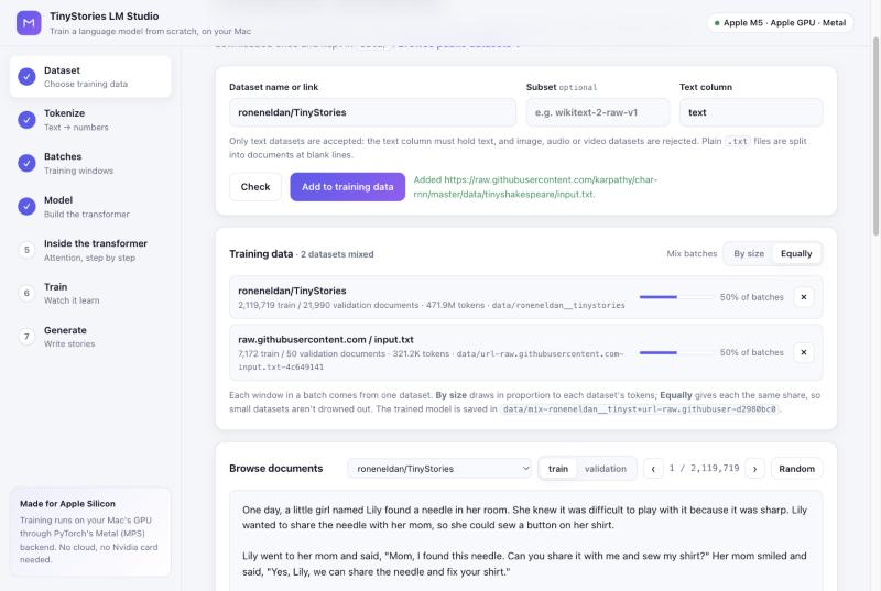 |
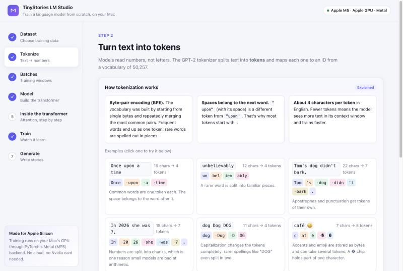 |
| Batches: a worked example | Pick a model size and see its parameter count |
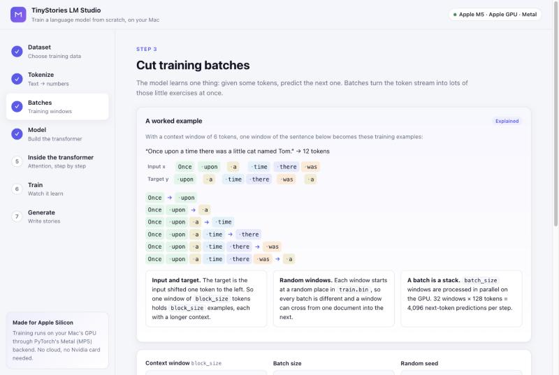 |
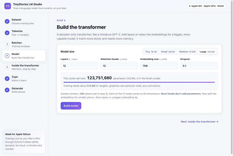 |
| The architecture, drawn from your settings | How every parameter adds up |
 |
 |
| Encoder, decoder, or both? | Attention weights after softmax, with the real model's heatmap |
 |
 |
| How a context vector is computed | Output projection, dropout and the residual connection |
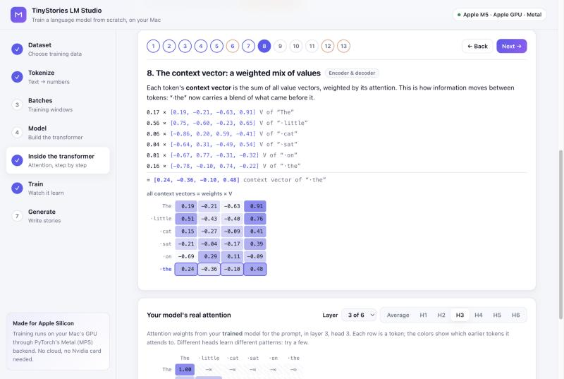 |
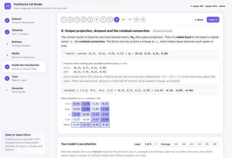 |
| The context vector goes through LayerNorm and the feed-forward network | Final LayerNorm, logits and softmax pick the next token |
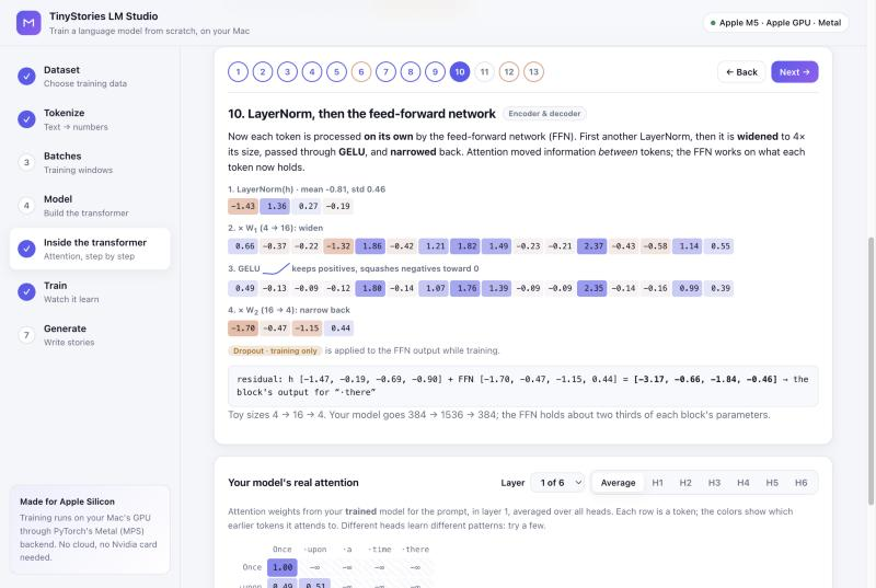 |
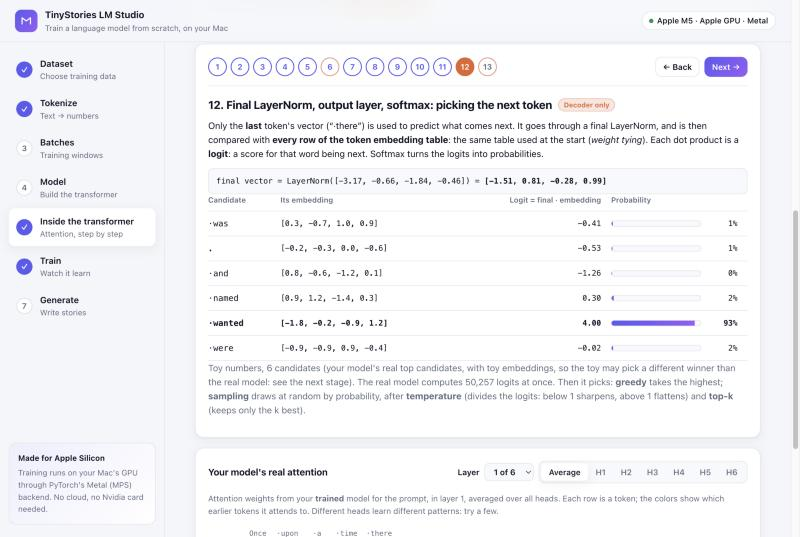 |
| Your real model's next-token probabilities | Generation with inference metrics |
 |
 |
| KV cache: with vs without | |
 |
|
| What one training step does | Training on a mix: updates, parameters updated, tokens |
 |
 |
Choosing datasets
TinyStories is the default, but any text dataset works, and you can train on several at once. A dataset can be given as:
| Form | Example |
|---|---|
| Hugging Face name | Salesforce/wikitext (plus subset wikitext-2-raw-v1) |
| Hugging Face link | https://huggingface.co/datasets/roneneldan/TinyStories |
| Link to a text file | https://raw.githubusercontent.com/karpathy/char-rnn/master/data/tinyshakespeare/input.txt |
File links can point to .txt, .jsonl, .json, .csv or .parquet files. GitHub page links are
converted to the raw file automatically. Plain .txt files are split into documents at blank lines.
From the command line:
python3 full-model.py --dataset Salesforce/wikitext --dataset-config wikitext-2-raw-v1
python3 full-model.py --dataset https://raw.githubusercontent.com/karpathy/char-rnn/master/data/tinyshakespeare/input.txt
python3 full-model.py --list-datasets
| Option | Meaning | Default |
|---|---|---|
--dataset |
Hugging Face name or link, or a link to a text file. Repeat it to train on several | roneneldan/TinyStories |
--dataset-config |
Subset name, for datasets that have them | none |
--text-column |
Column holding the text | text |
--mix |
With several datasets: size (in proportion to their tokens) or equal |
size |
--list-datasets |
Print the public datasets below with ready-to-run commands |
In the web app, enter the same values in step 1. In the notebook, they're the form fields in Step 1.
Training on several datasets
Each window in a batch is drawn from one dataset. By size picks datasets in proportion to their
tokens; equally gives each the same share, so a small dataset isn't drowned out (mixed by size, Tiny
Shakespeare would get only 0.07% of the batches next to TinyStories). In the command line, write a
dataset's subset and column as name@subset#column:
python3 full-model.py --mix equal \
  --dataset roneneldan/TinyStories \
  --dataset Salesforce/wikitext@wikitext-2-raw-v1 \
  --dataset https://raw.githubusercontent.com/karpathy/char-rnn/master/data/tinyshakespeare/input.txt
Text-only validation
Datasets are checked before anything is downloaded, using the dataset's metadata:
- Datasets with image, audio or video columns are rejected.
- The chosen column must exist and hold text (not numbers or labels). If it doesn't, the message lists the text columns that do exist.
- Datasets with several subsets list them so you can pick one (in the web app, as clickable buttons).
- Links must be reachable and point to a data file, not a web page.
- After downloading, the first rows are checked to make sure they hold readable text.
Public datasets that work out of the box
Each of these was checked with the validation above. The web app shows them as a gallery with Add and View buttons.
| Dataset | What it is | Size | Use with |
|---|---|---|---|
| Mini FineWeb-Edu | Educational web pages (the default, small subset; also debug, tiny, base, full) |
595K pages · 1.3 GB | --dataset BaoMinhTran/mini-fineweb-edu@small |
| TinyStories | Simple short stories | 2.1M stories · 1.0 GB | --dataset roneneldan/TinyStories |
| Tiny Shakespeare | A 1 MB selection of Shakespeare's plays | 1 text file · 1.1 MB | --dataset https://raw.githubusercontent.com/karpathy/char-rnn/master/data/tinyshakespeare/input.txt |
| WikiText-2 | Good and featured Wikipedia articles | 37K lines · 7.7 MB | --dataset Salesforce/wikitext@wikitext-2-raw-v1 |
| WikiText-103 | Over 100M tokens of Wikipedia | 1.8M lines · 315 MB | --dataset Salesforce/wikitext@wikitext-103-raw-v1 |
| Simple English Wikipedia | Every Simple English Wikipedia article | 242K articles · 157 MB | --dataset wikimedia/wikipedia@20231101.simple |
| WritingPrompts | Stories written for Reddit writing prompts | 273K stories · 605 MB | --dataset euclaise/writingprompts#story |
| TinyStories Instruct | TinyStories with instructions | 21.8M lines · 2.7 GB | --dataset roneneldan/TinyStoriesInstruct |
| CNN / DailyMail | News articles | 287K articles · 837 MB | --dataset abisee/cnn_dailymail@3.0.0#article |
| AG News | News headlines and descriptions | 120K articles · 20 MB | --dataset fancyzhx/ag_news |
| IMDB Reviews | Movie reviews | 25K reviews · 83 MB | --dataset stanfordnlp/imdb |
| Rotten Tomatoes | One-sentence review snippets | 8.5K sentences · 0.5 MB | --dataset cornell-movie-review-data/rotten_tomatoes |
Sizes are download sizes reported by Hugging Face. Find more on the Hugging Face datasets hub.
Where datasets are stored
Each dataset is downloaded once and kept in its own folder, with its own tokens and trained model, so
switching back and forth doesn't redo any work. A validation, valid, val or test split is used for
validation; if there isn't one, a small slice of train is held out.
data/
├── roneneldan__tinystories/
│   ├── dataset/               local copy of the downloaded dataset (~1.8 GB for TinyStories)
│   ├── train.bin              token IDs for training (~900 MB for TinyStories)
│   ├── validation.bin         token IDs for validation
│   ├── best_model_params.pt   best weights from training on this dataset
│   ├── model_config.json      model settings and training summary for those weights
│   └── runs.jsonl             history of every training run
└── mix-<datasets>-<hash>/     a model trained on several datasets (their tokens stay in their own folders)
data/ is git-ignored, so none of this is committed.
The Lab and the Journey
Two pages under Explore in the app's sidebar:
- Lab: start from a known design (GPT-2 style, Llama style, our best dense model, our best with experts,
or a fast and lean one) or set every switch yourself, each with what it measured in this project. A live
summary shows parameters (total and used per token), KV cache size and training memory. Pick one or more
tokenized datasets, the number of updates and the learning rate, and train: the run uses the same recipe as
ab_test.py(32 × 256-token updates, seed 42, four evaluations), then the model is evaluated and saved to the library with its full training record (models/<id>/training.json: settings, loss curves, speed). Compare models lists every model trained so far, grouped by the experiment that made it, and lines up any of them in one table: architecture, size and cost, quality and speed, with differences highlighted, the best value in each row in bold, and the validation and training curves overlaid. Recommend settings for me fills in the measured best choices for a goal (best quality, quality per compute, fastest generation, smallest KV cache), each marked with its reason; every decision and training setting (RoPE's base θ, the experts' balancing weight, warmup, final learning rate, weight decay, clipping, dropout) stays editable. Train this model asks where to train: on this Mac, or on Google Colab or Kaggle, for datasets not tokenized here (Mini FineWeb-Edu, for example) or for speed. A cloud run copies a run spec (every setting, plus optional comparison models) and openslab_run.ipynb; paste it, run all, and import the zip under Results from Colab or Kaggle. The same spec runs anywhere withpython3 ab_test.py --spec <spec>. OpenAI's GPT-2 small is in the library as a reference (python3 reference_gpt2.py --finewebdownloads it, prepares Mini FineWeb-Edu's held-out split and evaluates it); Against GPT-2 in the comparison lines it up with every model trained on FineWeb. - Journey: the best model at the top, the decisions that built it on one budget (2.631 → 2.200 after 1,000 updates), the numbers behind the model, and a timeline of every decision (wins, ties, losses and fixes), each with its result, the arithmetic behind it and its cost. Filter by area, or show only what's in the best model.
Saved models and evaluation
Training a new model on the same data used to replace the old one. Now every model you train (in the app or
with full-model.py) or import from Colab is also saved in a model library, models/<id>/, under its
own name, and is never overwritten. The app's Models step (step 8) lists them:
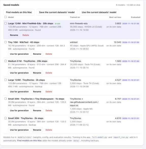
- Use for generation switches Generate and Inside the transformer to that model, whatever datasets
are selected. A model trained on Colab can be used without downloading its dataset. The choice is remembered
across restarts (
models/active.json). - Find models on this Mac adds the models already under
data/, including the backupsimport_run.pymade. Save the current datasets' model saves the one you're working with; training also saves the current model before replacing it. - Rename and Delete (which removes only the library copy;
data/isn't touched). - Quantize… opens the Quantize page for that model.
On the command line:
python3 registry.py scan        # add every model under data/ to the library
python3 registry.py list        # show the library
python3 -m quantization.checkpoint <model id> --bits 4   # save a round-to-nearest 4-bit copy in the library
Quantization: the Quantize page
The Quantize page (under Explore) stores a saved model's weights as small integers and compares the result with the original. Pick the model (its weight matrices are listed with their shapes), pick a recipe, and press Quantize and compare:
- Round to nearest, 8-bit or 4-bit (
quantization/rtn.py): every weight w ≈ q × scale; no data needed. The shared embedding / output layer stays at 8 bits. - GPTQ W4A16 (
quantization/gptq.py): llm-compressor'soneshoton our own model, wrapped as a Hugging Face model (quantization/hf_wrapper.py), calibrated on windows of a training-token file. The integers are read back into our own format, so the copy loads without llm-compressor.
The copy is saved in the model library (marked 8-bit, 4-bit or GPTQ 4-bit; use it on Generate, evaluate or benchmark it like any other), and the page shows both models' file and memory size, perplexity on every held-out set, and the same prompt continued by each (Generate on both for your own prompts). The 124M base model is 494 MB, 125 MB at 8 bits and 84–87 MB at 4 bits.
GPTQ needs llm-compressor, which pins its own torch and transformers, so it has its own environment; the app runs GPTQ there. Set it up once:
uv venv .venv-quant --python 3.11
VIRTUAL_ENV=.venv-quant uv pip install -r quantization/requirements.txt
.venv-quant/bin/python -m quantization.gptq <model id>          # GPTQ from the command line
.venv-quant/bin/python -m quantization.llm_compressor           # GPTQ on a stock Hugging Face model (Qwen3-0.6B)
The evaluation suite
Every model gets the same tests, so the numbers can be compared directly (evaluate.py):
- Held-out loss on every tokenized dataset on this Mac: 64 fixed windows of 256 tokens from each validation split, the same positions for every model. Loss is the average surprise per token; perplexity (eloss) is roughly how many tokens the model is choosing between.
- Generation: 6 fixed prompts (stories and educational text), 100 tokens each with a fixed seed, decoded greedy and with the Balanced preset. Measures how much greedy decoding repeats itself, the variety of the Balanced text, the model's confidence, speed with the KV cache and time to first token.
- Size: parameters, weights in memory and KV cache per token.
Results are stored with each model (models/<id>/eval.json). Tick models in the Models step and press
Evaluate selected models (15–40 seconds each on an M5), or:
python3 evaluate.py              # evaluate every saved model that hasn't been evaluated yet
python3 evaluate.py --table      # print the comparison table
All six models on this Mac, evaluated on an Apple M5:
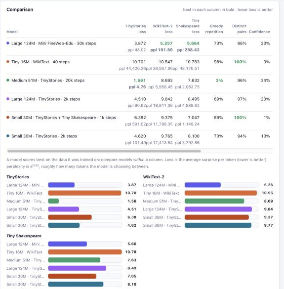
| Model | TinyStories | WikiText-2 | Tiny Shakespeare | Greedy repetition | Speed |
|---|---|---|---|---|---|
| Large 124M · Mini FineWeb-Edu · 30k steps | 3.872 | 5.257 | 5.664 | 73% | 49 tok/s |
| Medium 51M · TinyStories · 20k steps | 1.561 | 8.693 | 7.632 | 3% | 99 tok/s |
| Large 124M · TinyStories · 2k steps (old settings) | 4.510 | 9.842 | 8.495 | 69% | 60 tok/s |
| Small 30M · TinyStories · 2k steps (old settings) | 4.620 | 9.765 | 8.100 | 73% | 97 tok/s |
| Small 30M · TinyStories + Tiny Shakespeare · 1k steps | 6.382 | 9.375 | 7.047 | 89% | 98 tok/s |
| Tiny 16M · WikiText · 40 steps (a quick test) | 10.701 | 10.547 | 10.783 | 98% | 118 tok/s |
What it shows: each model is best on the kind of text it was trained on. The TinyStories model is excellent on stories (perplexity 4.8) and lost on Wikipedia, while the FineWeb model, trained on varied educational text, is the best on WikiText-2 and Shakespeare, neither of which it ever saw. The well-trained TinyStories model barely repeats itself even with greedy decoding (3%); the FineWeb model still loops greedily (73%), which is why the Balanced preset matters for it. The undertrained models, including the original 2,000-step runs, score far worse everywhere. (Mini FineWeb-Edu joins the held-out tests once it's downloaded and tokenized on this Mac.)
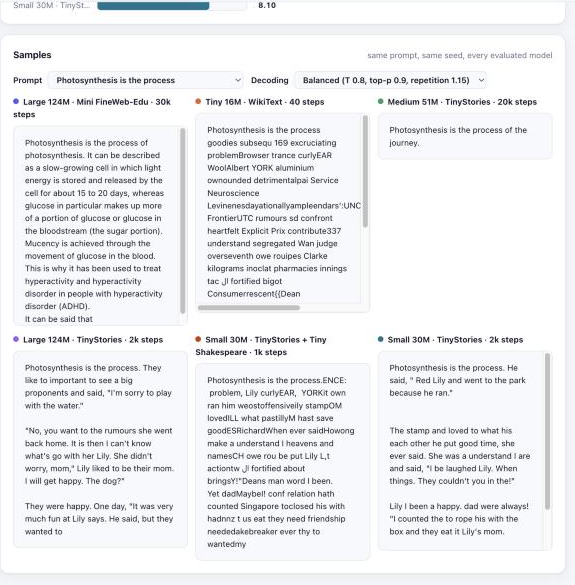
The Samples card shows every model's continuation of the same prompt side by side:
Standard benchmarks
The Benchmarks page (under Explore) runs the standard zero-shot tests used to compare language models:
| Test | What it tests | Questions | Chance |
|---|---|---|---|
| HellaSwag | picking the sensible ending of an everyday situation | 10,042 × 4 | 25% |
| LAMBADA | predicting the last word of a passage, which needs the whole passage | 5,153 | ≈0% |
| ARC-Easy | grade-school science questions | 2,376 | ~25% |
| PIQA | physical common sense, two options | 1,838 | 50% |
| Winogrande | filling a blank by common sense, two options | 1,267 | 50% |
benchmarks.py scores them the way EleutherAI's lm-evaluation-harness does (the same prompts and text clean-up):
each option is scored by how likely the model finds it after the question, and the most likely option is the
answer (accuracy; length-normalized accuracy divides by the option's length first). OpenAI's GPT-2 small,
loaded into this project's code, reproduces its published scores exactly (HellaSwag 28.92% / 31.14%, LAMBADA
32.56% and perplexity 40.06, ARC-Easy 43.81%, PIQA 62.89%, Winogrande 51.62%), which checks the scoring. Results
are saved with each model (models/<id>/benchmarks.json) and also shown on the Models page.
python3 benchmarks.py <model id>                         # all five, saved with the model
python3 benchmarks.py <model id> --tasks hellaswag,piqa  # some of them
python3 benchmarks.py <model id> --limit 200             # a quick check on 200 questions each (not saved)
A 124M model takes about 10 minutes for all five on an M5 (HellaSwag is most of it); the first run downloads the tests from Hugging Face. Models trained only on TinyStories score at chance: these tests need general knowledge. At GPT-2 size, scores sit close to chance, so compare them with the ± (one standard error) shown.
Facts the model knows: facts.py
The benchmarks measure reasoning and common sense; facts.py asks whether the model still knows simple facts
it read: 200 closed-book questions in evals/facts.jsonl (50 capitals, and science, geography, books and art,
history, everyday knowledge), each with three wrong answers of the same kind. It scores them two ways: by
likelihood like the benchmarks (choice: is "New Delhi" more likely than Mumbai, Kolkata and Bangalore after
"The capital of India is"?) and by letting the model answer on its own, greedily (generated: does the answer
appear?). A chat model gets the question in its chat format; a base model gets the plain sentence. Chance on
choice is 25%.
python3 facts.py <model id> [<model id> ...]           # saves models/<id>/facts.json, prints a table
python3 facts.py <chat model id> --as base             # a chat model on the plain sentences, as a base model
On 18 Nov it showed that instruction tuning had erased knowledge (the same numbers with the chat models on the plain sentences: 43% / −10.6 / 14%, so it isn't the format):
| Model | Choice (length-normalized) | Right answer's log prob | Generated |
|---|---|---|---|
| Base (stage 2) | 57.5% (52.5%) | −5.66 | 24% |
| Chat, SFT | 44.0% (45.0%) | −9.58 | 21% |
| Chat, SFT + DPO | 45.0% (44.0%) | −9.38 | 22% |
sft.py train now checks the facts (choice only) at every evaluation, and has two remedies: --lr (gentler steps)
and --replay 0.2 (a fifth of each batch is plain pre-training text from the base model's own datasets, made once
with python3 sft.py prepare-replay).
Redone that way (learning rate 5e-5, replay 0.2, 25 min on a Colab A100), instruction tuning keeps most of what the base model knew, at a small cost in how closely it matches the reference answers:
| Model | Facts (choice) | Right answer's log prob | Answered right | Benchmark average | Answer loss | Repetition (100 held-out) |
|---|---|---|---|---|---|---|
| Base | 57.5% | −5.66 | 24.0% | 41.5 | – | – |
| Chat, SFT (lr 2e-4) | 44.0% | −9.58 | 21.0% | 37.7 | 1.390 | 12.4% |
| Chat, SFT (lr 5e-5 + replay) | 50.0% | −7.17 | 25.5% | 40.3 | 1.448 | 15.6% |
| Chat, SFT (lr 2e-4) + DPO | 45.0% | −9.38 | 22.0% | 37.7 | – | 6.5% |
| Chat, SFT (lr 5e-5 + replay) + DPO | 50.5% | −7.07 | 30.0% | 40.5 | – | 8.5% |
(Benchmark average: length-normalized accuracy where a test has it, over the five.) DPO on the new model (2,000 fresh pairs from its own greedy answers, dpo.py pairs / train, 36 min on the Mac)
brings repetition down from 15.6% to 8.5% and answers that end from 73% to 82%, while keeping the knowledge: it is the
best chat model of 18 Nov.
(Correction, 19 Nov: the held-out repetition and endings above were measured with dpo.py eval's default pairs file,
data/dpo-pairs.jsonl, whose 100 held-out questions are not held out from the D1b DPO pairs: 80 of them were
training pairs. On the D1b file's own held-out 100, which neither model trained on: SFT (lr 5e-5 + replay)
repetition 16.0%, ended 69%; with DPO 8.5%, 87% (answer loss 1.230 → 1.333). The old chat model (2746ba) gets
7.5% and 85% there, but 48 of those questions were in its own DPO pairs. Since 19 Nov this file is
dpo.py eval's default (dpo.EVAL_PAIRS), and serving/check.py uses the same 100 questions.)
A reward model as the judge: bestofn.py
DPO's pairs so far set the dataset's reference answer against the model's own greedy one. A reward model can
instead judge the model's own answers: sample several, keep the best and the worst. bestofn.py does this locally
with Skywork-Reward-V2-Qwen3-0.6B (Apache-2.0,
1.2 GB): a sequence classifier that gives one score to a (question, answer) pair.
python3 bestofn.py --model <chat model id> [--n 6] [--temperature 0.5]   # pilot: judge's pick vs greedy
python3 bestofn.py --model <chat model id> --pairs 2000 --temperature 0.5 # → data/dpo-pairs-rm.jsonl
python3 dpo.py train --model <chat model id> --path data/dpo-pairs-rm.jsonl [--method simpo]
The pilot (300 questions: the 100 held-out chat questions and the 200 fact questions; greedy and 6 samples each) asks whether the judge's pick beats greedy decoding at all. At temperature 0.8 it doesn't: the samples are much worse than greedy (facts answered right 14.5% vs 30%) and the best of 6 still loses (26.5%). At 0.5 it does: the judge's best of greedy + 6 answers 37% of the fact questions right (greedy 30%; some answer is right for 43%), with a higher judge score (−2.87 vs −5.43) and half the repetition. The judge ranks a right answer above a wrong one in 76% of pairs and doesn't favour long answers (length and score correlate at −0.2 to −0.4); it does sometimes prefer a short confident wrong answer.
The pairs: 2,000 new smol-smoltalk questions (none from earlier pair files), greedy + 6 samples at 0.5, the judge's best as chosen and its worst as rejected, both the model's own tokens (1,999 pairs; median score gap 5.0; the greedy answer was chosen in 20%). Chosen answers repeat less (4.8% vs 9.0%), end more often (93% vs 69%) and are shorter (119 vs 140 tokens; the chosen one is the longer in only 30% of pairs).
Training on them (2 epochs, lr 2e-6, about 17 minutes each on the Mac), DPO against a frozen reference (beta 0.1)
and SimPO (--method simpo: no reference model; each answer's reward is its mean log probability per token,
and the chosen must win by a margin: beta 2.0, gamma 1.0). On the 100 held-out D1b questions:
| Model | Repetition | Ended | Length | Answer loss | Facts (choice) | Answered right | Benchmark average |
|---|---|---|---|---|---|---|---|
| SFT (lr 5e-5 + replay) + DPO (4c0ef4) | 8.5% | 87% | 127 | 1.333 | 50.5% | 30.0% | 40.5 |
| + DPO on reward-model pairs (e45919) | 2.3% | 99% | 99 | 1.425 | 50.5% | 31.0% | 40.5 |
| + SimPO on reward-model pairs (0881b0) | 2.2% | 99% | 95 | 1.474 | 49.5% | 27.0% | – |
DPO on the judge's pairs makes the answers clean (a quarter of the repetition, nearly all end) and keeps the knowledge and the benchmarks (HellaSwag 33.0, LAMBADA 14.4, ARC-Easy 44.4, PIQA 61.7, Winogrande 48.9): it is the best chat model, and the served one since 19 Nov. The answer loss rises because the model now writes shorter answers in its own style rather than the dataset's. SimPO cleans up as well but loses a few facts; at this learning rate it barely moved (its held-out margin stayed below gamma), so it might do better with a larger one. The 37% of the best-of-7 pilot didn't carry over into training (31%): the pairs mostly teach style, not facts.
Asking several times: selfconsistency.py
Some answer among seven is right for 43% of the fact questions, against 31% for greedy. Self-consistency asks the
model several times and chooses among its answers, with no training. selfconsistency.py takes the greedy answer
and N − 1 samples (temperature 0.5) per fact question and compares choosers over the first k answers: a vote on
what each answer names (the words after the question's stem, "The capital of India is | New Delhi"), the model's own
confidence (highest mean log probability per token), the vote with confidence as tie-break, the judge
(the reward model's favourite), and the oracle (right if any answer is right: the ceiling). The choosers never see
the right answer.
python3 selfconsistency.py --model <chat model id> [--n 11] [--temperature 0.5] [--no-judge]
On the served chat model (e45919, 19 Nov), facts answered right out of 200:
| k answers | Greedy | Vote | Confidence | Vote + confidence | Judge | Oracle |
|---|---|---|---|---|---|---|
| 1 | 31.0% | 31.0% | 31.0% | 31.0% | 31.0% | 31.0% |
| 3 | 31.0% | 31.0% | 31.5% | 30.5% | 34.5% | 40.0% |
| 5 | 31.0% | 31.5% | 28.5% | 31.0% | 34.0% | 43.5% |
| 7 | 31.0% | 31.0% | 29.5% | 30.0% | 36.5% | 46.0% |
| 11 | 31.0% | 30.0% | 29.5% | 29.5% | 37.0% | 48.5% |
Voting doesn't help. It finds the right answer only when that answer is the most common one, and where greedy is wrong it rarely is: in the 35 questions with greedy wrong and some answer right, a median of 2 of the 11 answers are right (only one in 15 of them), and wrong answers repeat too (India's capital: "Kedarnath" and "New York City" four times each, "Delhi" once). The model's confidence doesn't separate right from wrong either. The judge helps (+6 points with 9–11 answers, about 1.4 s per question for 11 answers on the Mac), but Qwen3-0.6B is a much stronger model: the gain is its knowledge, not the 124M model's. What the model gets wrong it mostly doesn't know firmly, so choosing among its own answers can't fix it; more or better pre-training, or retrieval (the facts in the prompt), would.
Everything at once: the evaluation queue
One command evaluates a model end to end. It can be stopped at any point; running it again continues with the
next task (infra/eval_queue.py):
python3 -m infra.eval_queue f6-124m-stage2-2p5b          # a diffusion run: bound, quality, the five benchmarks
python3 -m infra.eval_queue <model id>                   # an autoregressive model: the suite, the five benchmarks
python3 -m infra.eval_queue <target> --quick             # 20 questions per benchmark, nothing saved: a check
python3 -m infra.eval_queue <target> --plan              # what's done and what's left
python3 -m infra.eval_queue <target> --only bench:hellaswag --redo
Each task's state (done, failed, minutes, batch size) is kept in eval_queue.json in the model's folder. The scoring
batch size is chosen from the free GPU memory and halved if a task still runs out of memory. On macOS the queue
keeps the Mac awake with caffeinate. A 124M diffusion model takes about 3 hours, two of them on HellaSwag.
The results store
Every evaluation also adds its numbers to one file, results/results.jsonl (committed):
one record per measurement, with the model, the settings, when it was measured and at which commit. The evaluation
suite, benchmarks.py, sft.py compare, dpo.py eval, and the diffusion model's benchmarks.py and quality.py
do this by themselves, and docs/results.md, a page of every model's latest numbers, is regenerated
from it. Results measured on Colab arrive with the model: python3 -m infra.model_store pull <repo> adds them.
python3 -m infra.results scan              # add the result files already in models/, diffusion_models/runs/, outputs/
python3 -m infra.results show <model id>   # the latest numbers of one model
python3 -m infra.results render            # regenerate docs/results.md (the tests fail if it's out of date)
The app serves the records at /api/results (?model=<id>&kind=benchmark, or all=true for every measurement).
Writing text, step by step
The Writing text page (under Explore) shows how a model produces a continuation: one token per step, left to right, one pass through the model each. Pick a model (the base model by default) and a prompt, then play the generation back: each token is shaded by the model's confidence, a card shows the top five candidates at that step, and a step × position grid shows which position each step wrote (for left-to-right writing, a staircase). The prompts are the openings of 8 held-out documents (4 FineWeb-Edu, 4 TinyStories), so the page also shows the real continuation, shaded by how surprised the model was by each real token.
Run the prompt set generates 64 tokens (greedy) after each prompt and saves the averages with the model
(models/<id>/textgen.json): steps, loss and top-1 accuracy on the real continuation, confidence, speed and
repetition. The prompts, tokenizer and length are fixed, so other ways of generating text can later be compared on
the same footing. On the base model: loss 3.481 on the real continuations (GPT-2 small 3.118), and 28% repeated
4-token runs in greedy text (GPT-2 61%).
The website
pages/build.py builds the project's website into _site/. It has the docs as pages, the Journey timeline, the
Explorer (the base model's real numbers for three saved prompts) and a Side by side replay, which run in the browser
from saved data, and Try it, which runs the real 124M chat or base model in the browser: it downloads the 8-bit
GGUF from the Hugging Face repos (174 MB, cached) and generates with wllama
(llama.cpp in WebAssembly). After each answer it shows llama.cpp's own timings (time to first token, prefill and decode
speed, compute and memory rates, KV cache reuse), the time of every token, and where the model runs; switch between
the GPU (WebGPU) and the CPU to compare. On every push to main that changes the docs,
.github/workflows/pages.yml builds it and deploys it to GitHub Pages.
python3 pages/build.py && python3 -m http.server 8090 -d _site       # build, then open http://localhost:8090
python3 pages/record.py                                              # re-record the Explorer and side-by-side runs (needs the app running)
python3 pages/record.py --only explorer                              # just the Explorer, on the model in use (pick the base model first)
Serving: export as a standard Hugging Face model
serving/export_hf.py turns one of our models into a standard Hugging Face Qwen3 folder, so tools that serve
Qwen3 (transformers, llama.cpp through GGUF, MLX, LM Studio, Ollama, vLLM) can run it with no code of ours:
python3 -m serving.export_hf mini-fineweb-edu-ful-202611151103-bb160c      # the base model → exports/<id>-qwen3/
python3 -m serving.export_hf chat-mini-fineweb-ed-202611152150-2746ba      # the DPO chat model, with its chat template
It checks the export against our model before saving (largest logit difference, the top token at every position,
greedy text) and writes the result into export_info.json. Our design is Qwen3's except that the block norms are
LayerNorm; the export centers the residual stream so LayerNorm and RMSNorm give the same result, and scales the query
and key projections so Qwen3's single epsilon acts like our QK-norm's. Load it like any model:
from transformers import AutoModelForCausalLM, AutoTokenizer
tok = AutoTokenizer.from_pretrained("exports/chat-mini-fineweb-ed-202611152150-2746ba-qwen3")
model = AutoModelForCausalLM.from_pretrained("exports/chat-mini-fineweb-ed-202611152150-2746ba-qwen3")
ids = tok.apply_chat_template([{"role": "user", "content": "Why is the sky blue?"}], add_generation_prompt=True, return_tensors="pt")
print(tok.decode(model.generate(ids, max_new_tokens=80)[0, ids.shape[1]:], skip_special_tokens=True))
To serve it with llama.cpp (Homebrew's llama.cpp), make a GGUF file and start llama-server, which speaks the
OpenAI API (/v1/chat/completions with the chat template, /v1/completions, streaming). The script fetches only
llama.cpp's converter the first time:
serving/gguf.sh exports/chat-mini-fineweb-ed-202611152150-2746ba-qwen3 fineweb-edu-124m-chat-dpo   # → exports/gguf/*-bf16.gguf, *-Q8_0.gguf
llama-server -m exports/gguf/fineweb-edu-124m-chat-dpo-Q8_0.gguf --jinja -c 512 --port 8080
curl localhost:8080/v1/chat/completions -H 'Content-Type: application/json' \
  -d '{"messages": [{"role": "user", "content": "What is the capital of France?"}], "temperature": 0}'
On the M5 that's about 256 tokens/s in bfloat16 and 377 in 8 bits, with the same greedy text as our own code. LM Studio and Ollama load the same GGUF files.
Both are published in these formats: fineweb-edu-124m-base-qwen3
and fineweb-edu-124m-chat-dpo-qwen3, so no export is
needed to run them: llama-server -hf aramkris/fineweb-edu-124m-chat-dpo-qwen3:Q8_0 --jinja -c 512, or
ollama run hf.co/aramkris/fineweb-edu-124m-chat-dpo-qwen3:Q8_0. serving/publish.py <export> <gguf name> <repo>
uploads a new one (card from docs/model_cards/<repo>.md).
serving/check.py checks that the served model is the model (S7). engine runs our own held-out loss and benchmark
code with llama.cpp computing the numbers (through llama-cpp-python: uv pip install --python .venv/bin/python
llama-cpp-python); api starts llama-server and sends LAMBADA and, for chat models, dpo.py eval's 100 held-out
questions over HTTP, next to our own model on the same questions:
.venv/bin/python -m serving.check engine exports/gguf/fineweb-edu-124m-base-bf16.gguf --model mini-fineweb-edu-ful-202611151103-bb160c
.venv/bin/python -m serving.check api exports/gguf/fineweb-edu-124m-chat-dpo-bf16.gguf --model chat-mini-fineweb-ed-202611152150-2746ba
| Served by llama.cpp | Held-out FineWeb-Edu | Benchmark average | LAMBADA over HTTP | Chat: repetition / ended / length |
|---|---|---|---|---|
| Our PyTorch model (stored) | 3.2957 | 42.35 | 20.34% | 6.5% / 86% / 129.1 |
| bfloat16 GGUF | 3.2959 | 42.34 | 20.36% | 6.6% / 85% / 129.1 |
| 8-bit GGUF (Q8_0) | 3.2963 | 42.22 | – | 6.7% / 82% / 133.2 |
Generating text from a trained model
The web app's Generate step does this for you. Its model list also has the masked diffusion runs: pick one and the page writes the whole continuation at once, replaying the denoising passes (choose 16 to 128 passes, which tokens stay and the block size). From Python:
from data import dataset_paths
from inference import generate_text, load_model, load_model_config
from tokenization import get_tokenizer
from train_config import setup_device

paths = dataset_paths("roneneldan/TinyStories")          # same name (and subset) you trained on
config, info = load_model_config(paths.model_config)
dev = setup_device()
model = load_model(config, paths.checkpoint, dev.device)

print(generate_text(model, get_tokenizer(), "Once upon a time there was a dragon who",
                    dev.device, max_new_tokens=200, temperature=0.8, top_k=50))
temperature: lower is more predictable, higher is more varied.top_k: only sample from thekmost likely next tokens (Nonefor no limit).
For a model trained on several datasets, use mix_paths([...dataset folders...]) from data.py instead of
dataset_paths.
Resuming and extending a run
Every evaluation saves the full training state next to the model, in training_state.pt: the latest
weights, AdamW's running averages for every parameter, the mixed-precision scaler, the step, the loss history
and the random-number state, with a small summary in training_state.json. A run can then carry on later:
- Finish an interrupted run. Continuing with the same number of steps picks up at the step where the state was saved, with the same weights, optimizer state and learning-rate schedule (after stopping in the app, closing the terminal, or a disconnected Colab session).
- Extend a finished run. Asking for more steps stretches the cosine learning-rate schedule to the new end. A finished run has decayed to the minimum learning rate, so instead of crawling on at the minimum, the learning rate ramps back up to the stretched curve over a short re-warmup (200 steps, or a fifth of the extension if that's shorter) and then decays again. Extending a 30,000-step run to 40,000, it ramps from 6e-5 to 1.4e-4 and returns to 6e-5 at step 40,000.
Every run now also ends with a final evaluation, so the last stretch of training counts towards the best checkpoint, and a run shorter than one evaluation interval still saves its model.
Where to continue a run:
| Where | How |
|---|---|
| Web app | Continue training in the Train step: shows the saved run (step, best loss, learning rate) and trains until the step you choose |
| Command line | python3 full-model.py --resume [--max-iters N] |
| Colab / Kaggle | Tick resume in Step 5. Files in /content disappear when a Colab session disconnects, so for long runs tick keep_checkpoints_in_drive to save the checkpoints and training state in Google Drive |
| Colab → Mac | Tick include_training_state in Step 10; import_run.py installs it, and the run continues on the Mac |
The training state is about three times the size of the weights (the weights plus AdamW's two running averages), e.g. about 1.5 GB for the 124M Large model.
Configuration
Diffusion: writing by denoising
The Diffusion page (under Explore) runs the masked diffusion models from diffusion_models/ (train one with
diffusion_models/diffusion_colab.ipynb, then unzip it into diffusion_models/runs/<name>/). The continuation
starts as all [MASK] (█); every step is one pass through the model, reading the whole text in both directions,
and a few masked positions are revealed. Pick a model, a prompt (the same held-out prompts as Writing text), the
number of tokens and steps, and how positions are chosen (confident first with a repetition penalty of 1.3 by
default; also no penalty, blocks of 8 left to right, random order, or v1's re-sampling), then play it back. A grid
shows when each position was revealed: scattered clusters instead of the left-to-right staircase. Below, a table
compares the trained runs: size, training tokens and time, the likelihood bound, and the scores from
python3 -m diffusion_models.quality <run> (the base model's loss on the generated text, and repetition).
Side by side: autoregressive vs diffusion
The Side by side page (under Explore) gives one prompt to an autoregressive model (the base model by default) and a diffusion run (by default the 124M one trained on the same data and number of tokens). It replays both together, lined up by model pass or by clock time. Each lane has its own grid of which position each pass writes: a staircase for the autoregressive model, blocks or scattered clusters for diffusion, with the same row height so the heights compare the number of passes. Both texts are scored the same way: passes, time, tokens per second, the base model's loss on the text, repetition, and the loss on the real continuation (exact for the autoregressive model, the likelihood bound for diffusion). Below, a table sets out what differs: attention, the training objective, the cost of a pass.
Model size: full-model.py
config = GPTConfig(
    vocab_size=50257,   # GPT-2 tokenizer
    block_size=256,     # context window (tokens)
    n_layer=6,          # transformer blocks
    n_head=6,           # attention heads per block
    n_embd=384,         # embedding size
    dropout=0.0,
    bias=True
)
Training: train_config.py
| Setting | Default | Meaning |
|---|---|---|
max_iters |
20000 | Training steps |
learning_rate |
6e-4 | Peak learning rate |
min_lr |
6e-5 | Learning rate at the end of the cosine decay |
warmup_steps |
1000 | Steps of linear warmup |
batch_size |
32 | Sequences per batch |
gradient_accumulation_steps |
1 | Batches averaged per optimizer update (1 = update every step) |
eval_interval |
1000 | Evaluate every N steps |
eval_iters |
100 | Batches per evaluation |
weight_decay |
0.1 | AdamW weight decay |
grad_clip |
1.0 | Gradient norm clipping |
The web app's Quick preset uses 2,000 steps, 200 warmup, and evaluation every 250 steps over 50 batches, with the same learning rate and no gradient accumulation. Full uses the defaults above. See Getting better stories for why these settings replaced the original ones.
Train on a cloud GPU: Google Colab or Kaggle
Everything runs on your Mac except, if you like, the training itself. The notebook
train_step_by_step.ipynb runs on Google Colab or Kaggle, trains on their
Nvidia GPU, and packages the result into one zip that you bring back with import_run.py.
On a GPU the notebook also shows:
- the GPU's name, memory and utilization (
nvidia-smi); - a model size dropdown up to Large (124M parameters, GPT-2 small size), which fits easily on a T4;
- training throughput (tokens per second) and peak GPU memory after training;
- Step 9: a KV cache benchmark at several lengths (tokens per second with and without the cache, cache size, rebuilds once the window is full, GPU memory);
- Step 10: everything packaged into
tinystories-run-<dataset>-<date>.zip.
CUDA GPUs train with mixed precision: bfloat16 on GPUs with native support (compute capability 8.0+, such as A100 and L4), float16 with a gradient scaler otherwise (such as the T4).
Google Colab
- Open the notebook in Colab: Open in Colab (also the badge at the top of the README).
- Runtime → Change runtime type → T4 GPU (free), or L4 / A100 with Colab Pro or compute units.
- Run the cells from top to bottom. Step 0 clones this repository and installs the dependencies.
- Set the run with the form fields: the dataset (Step 1),
model_size(Step 4, e.g.large) andmode(Step 5:quickorfull). - Step 10 downloads the results zip to your computer (allow the download if the browser asks). It's also in the Files panel.
Things to know on Colab:
- "This notebook was not authored by Google". Colab shows this warning for any notebook opened from GitHub. The notebook doesn't mount Google Drive or ask for your Google data; choose Run anyway.
- Running everything except the download. To run the whole notebook but decide later whether to download the zip, select the Step 10 cell and use Runtime → Run before. Run Step 10 when you're ready.
- Changing code mid-session. Step 0 runs
git pullwhen the repository is already cloned. After pulling new code, use Runtime → Restart session (files in/contentare kept) so Python loads it. - Precision. GPUs with native bfloat16 (compute capability 8.0+: A100, L4) train in bfloat16. Older GPUs such as the T4 train in float16 with a gradient scaler: the T4 reports bfloat16 as supported, but only through slow emulation (1.4 s per step for the Large model, versus about 3.9 steps per second in float16).
- Sessions. Free Colab sessions can disconnect when idle or when usage limits are reached, and files in
/contentare lost when they do. On Colab Pro, GPU time uses compute units.
The numbers from a real run on a free Colab T4 are in Analysis: Measured on a Colab T4.
Kaggle
- On kaggle.com, Create → New Notebook, then File → Import Notebook and paste
the link to
train_step_by_step.ipynbon GitHub. - In the side panel, Settings → Accelerator → GPU (T4 or P100; one GPU is used) and switch Internet on, which Kaggle only allows for phone-verified accounts.
- Run the cells from top to bottom. The Colab form fields appear as plain variables you can edit. The code
and data go to
/tmp, so only the results zip is saved as the notebook's output. - Download the zip from the Output panel (
/kaggle/working). Save Version → Save & Run All runs the whole notebook in the background, so you can close the tab.
Kaggle sessions run for up to about 12 hours, with a weekly GPU quota (around 30 hours at the time of writing; your account page shows the current limit).
Bring the model home
From the project folder on your Mac:
python3 import_run.py ~/Downloads/tinystories-run-roneneldan__tinystories-20261110-1430.zip
It puts the weights and config in data/<dataset>/ (backing up the model already there to
data/<dataset>/backups/), adds the run to the training history, and keeps the loss chart, GPU metrics and
sample story in data/<dataset>/imported/. Start python3 app/server.py and the Generate and Inside the
transformer steps use the GPU-trained model. If that dataset isn't on your Mac yet, add it in the Dataset
step first.